Wednesday 28 March 2012

Lab 4 (Part 2) : Intensity Transformation and Spatial Filtering

For this week, our lab is more focusing on Spatial Filtering.


Spatial filtering term is the filtering operations that are performed directly on the pixels of an image. The process consists simply of moving the filter mask from point to point in an image. At each point (x,y) the response of the filter at that point is calculated using a predefined relationship. (reference from Google Doc)

There are two main types of filtering applied to images:
    - Spatial domain filtering
    - Frequency domain filtering

To give further ideas on how spatial filtering is applied to an image, the following MATLAB code was written by Nova Scheidt:


For you to apply the filter to the MATLAB code above, the following calls are made:


Monday 26 March 2012

Lab 4 (Part 1) : Intensity Transformation and Spatial Filtering

In today's lab (20/3/2012), we have learnt about Intensity. This lab is divided into several category. All category will be elaborate afterwards.


1. Intensity Transformation Function
When you are working with gray-scale images, sometimes you want to modify the intensity values. For instance, you want to reverse the black and the white intensities or you may want to make the dark darker and the lights lighter.

Generally, making changes in the intensity is done through Intensity Transformation Function. Next section talks about four main intensity transformation functions:

        a. photographic negative (using imcomplement)
        b. gamma transformation (using imadjust)
        c. logarithmic transformations (using c*log(1+f))
        d. contrast-stretching transformations (using 1./(1+(m./(double(f)+eps)).^E))

a.    Photographic Negative
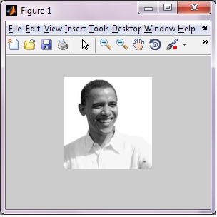
The Photographic Negative is probably the easiest of the intensity transformation to describe. Assume that we are working with grayscale where black is 0 and white is 1. The idea is black become 1 and white become 0 and any gradient in between are also reserved. In intensity, this means that the true black become tru white and vise versa .


Original
                                                                       
Photographic Negative
                                                             
b.   Gamma Transformation
With gamma transformation, you can curve the gray scale component either to brighten the intensity (when gamma is less than one) or darker the intensity (when gamma is greater than one).


Original (gamma = 1)

gamma = 3

gamma = 0.4


c.    Logarithmic Transformation
Logarithmic transformation can be used to brighten the intensities of an image (like the Gamma Transformation, where gamma<1). More often, it is used to increased the detail (or contrast) of lower intensity values.

Original

C = 1

C = 2

C = 5


d.    Contrast-stretching Transformation
Contrast-stretching Transformation  result in increasing the contrast between the darks and the lights. Effectively, what you end up with is the dark being darker and the lights being lighter, with only few level of gray in between.


Original

E = 4

E = 5

E = 10


2. Spatial Filtering
Spatial filtering is a technique that you can use to smooth, blur, sharpen or find the edge of an image. The following four images are meant to demonstrate.


a. Zero-Padded
Zero padding is the default. You can also specify a value other than zero to use as padding value.


b. Replicate


c. Symmetric


d. Circular


e. Special Filter


     i) Motion picture


     ii) Sharpening
The principal objective of sharpening is to highlight fine detail in an image or to enhance detail that has been blurred, either in error or as an natural effect of a particular method of image acquisition.


     iii) Horizontal edge-detection


Saturday 17 March 2012

Lab 3 - Part 2

Image Acquisition and Basic Operation (MATLAB)

For this topic, the learning objective is to learn basic operations related to image acquisition.

1.      Read and display image
To read the image, use imread command, but make sure the image file is in a correct path (refer figure below, in the red rectangle).


2.      Convert image into grayscale
To convert color image into grayscale, use rgb2gray command.


3.      Display image into green channel


The above command and resulting image shows the intensity of green color in the original image data.

4.      Image transpose
To transpose the image A, use “ ‘ ” sign at the end of variable, example: A’


5.      Image cropping


The imcrop command creates an interactive Crop Image tool associated with the image displayed in the current figure, called the target image. The Crop Image tool is a moveable, resizable rectangle that can be position interactively using the mouse. When the Crop Image tool is active, the pointer changes to cross hairs " + ", when moving it over the target image. Using the mouse, specify the crop rectangle by clicking and dragging the mouse. Use mouse to move or resize the crop rectangle. When finish sizing and positioning the crop rectangle, create the cropped image by double-clicking the left mouse button or by choosing Crop Image from the context menu. Use imshow command to display the crop image.

6.      Flip vertical
Use fliplr command to flip the image from left to right. However, it should be noted that fliplr command only work for 2-D matrices. 


Tuesday 13 March 2012

Lab 3 - Part 1

Image Processing Toolbox Tutorial

In today's lecture, we learned some basic topic about Image Processing and Pattern Recognition using Matlab Tool. This tutorial consist of:


  1. Read and display an Image
  2. Check how the image appear in the workspace
  3. Perform histogram equalisation on the image
  4. Write the image to a disk file
  5. Get info about graphic file

1. Read and display image
To read an image, use imread command. Lets read the image in PNG format and show the image on your workspace by using imshow command


2. Check the image memory
Enter the whos  command to see how the I variable stored in the library.


3. Perform histogram equalisation


As you can see, pout2.png is a low contrast image. To see the distribution of intensities in pout2.png in its current state, you can create a histogram by calling the imhist function.


Notice how the intencity range is rather narrow

Now call histeq(I) to spread the intensity values over the full range, thereby improving the contrast of I. Return the modified image in variable I2


Display the new equalised image, I2 using this command. 


Call imhist again this time for I2


4. Write the Image
Write the newly adjusted image I2 back to disk. Let say you like to save it as TIF file. Use imwrite and specify the filename includes the extension 'tif'


5. Check the content of the newly written file
Use imfinfo function to see what was written to the disk.


Now you have two same image with different format.