Car Plate Recognition

There have been several months since the last post. Now, I’m working into a new project which is car plate recognition. So, has anyone here know how to do this? Well, I hope there will be some comments for this posting. J At least we can share the idea right?? So, help me… Thank you.

Color Segmentation

For this week, we had learn about color segmentation. The aim for this lab is to identify different colors in fabric by analyzing the L*a*b* colorspace. The fabric image was acquired using the Image Acquisition Toolbox.

Now, we will explain about how to segment the color in an image.

Steps:

• 
  
• Step 1: Read Image
  Step 2: Calculate Sample Colors in L*a*b* Color Space for Each Region
  Step 3: Classify Each Pixel Using the Nearest Neighbor Rule
  Step 4: Display Results of Nearest Neighbor Classification
  Step 5: Display 'a*' and 'b*' Values of the Labeled Colors. 
• 
  

Step 1 : Read Image


For this lab, we used the image as below:

                                                                               fabric.png

Read in the fabric.png image, which is an image of colorful fabric.

Step 2: Calculate Sample Colors in L*a*b* Color Space for Each Region

From the above image (fabric.png), we can see that there are six colors which is black, red, green, yellow, purple and magenta. We can simply names all the color in that image, but using the L*a*b colorspace will enable us to quantify these visual differences.

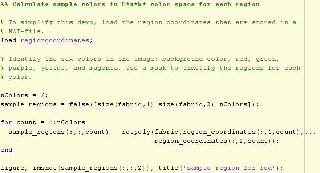
The L*a*b* space consists of a luminosity 'L*' or brightness layer, chromaticity layer 'a*' indicating where color falls along the red-green axis, and chromaticity layer 'b*' indicating where the color falls along the blue-yellow axis.

Next, we will choose a small sample region for each color in the image and calculate each sample region's average color in 'a*b" space. We will use these color markers to classify each pixel.

To convert image from RGB color space to L*a*b* color space, use the code below:

Calculate the mean 'a*' and 'b*' value for each area that we extracted and these values serve as our color markers in 'a*b*' space.

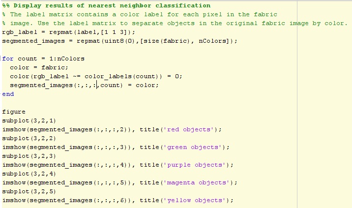
Step 3: Classify Each Pixel Using the Nearest Neighbor Rule

Each color marker now has an 'a*' and a 'b*' value. We can classify each pixel in the lab_fabric image by calculating the Euclidean distance between that pixel and each color marker. The smallest distance will tell us that the pixel most closely matches that color marker. For example, if the distance between a pixel and the red color marker is the smallest, then the pixel would be labeled as a red pixel.

Create an array that contains your color labels, i.e., 0 = background, 1 = red, 2 = green, 3 = purple, 4 = magenta, and 5 = yellow.

Step 4: Display Results of Nearest Neighbor Classification

Step 5: Display 'a*' and 'b*' Values of the Labeled Colors. 

To be more focus, let see each output below:

References:
1) http://www.mathworks.com/products/image/examples.html?file=/products/demos/shipping/images/ipexfabric.html
2) http://www.mathworks.com/products/demos/image/color_seg_k/ipexhistology.html

Region Segmentation

Hai, we meet again in this new post..

In conjunction with Labor Day next week, Image Processing class has been cancelled. But, our lovely lecturer has an ASSIGNMENT for us on that HOLIDAY.

Thus, in this post, we gonna discuss about REGION SEGMENTATION.

What is a Region?

•  Basic definition : a group of connected pixels with similar properties.
•  Important in interpreting an image because they may correspond to objects in a scene.
•  For correct interpretation, image must be partitioned into regions that correspond to objects or parts of an  object.

What is Segmentation?

• Another way of extracting and representing information from an image is to group pixels together into regions of similarity. 
• If an image has been preprocessed appropriately to remove noise and artifacts, segmentation is often the key step in interpreting the image. 
• Image segmentation is a process in which regions or features sharing similar characteristics are identified and grouped together.
• Image segmentation may use statistical classification, thresholding, edge detection, region detection, or any combination of these techniques. 
• The output of the segmentation step is usually a set of classified elements.
• Most segmentation techniques are either region-based or edge-based.

• Edge-based techniques rely on discontinuities in image values between distinct regions, and the goal of the segmentation algorithm is to accurately demarcate the boundary separating these regions.

• Region-based techniques rely on common patterns in intensity values within a cluster of neighboring pixels. 
• The cluster is referred to as the region, and the goal of the segmentation algorithm is to group regions according to their anatomical or functional roles.
• Important principles:- 
•   Value similarity - Gray value differences 
                                  - Gray value variance


• Spatial Proximity - Euclidean distance 
                                            - Compactness of a region


• Region-based segmentation methods attempt to partition or group regions according to common image properties. These image properties consist of : 

1. Intensity values from original images, or computed values based on an image operator
2. Textures or patterns that are unique to each type of region
3. Spectral profiles that provide multidimensional image data

• Elaborate systems may use a combination of these properties to segment images, while simpler systems may be restricted to a minimal set on properties depending of the type of data available.

• There are three basic approaches to segmentation:
• Region Merging - recursively merge regions that are similar.

                                       Original image                             Region Merging
                          

                                      Original image                              Region Merging


• Combine regions considered similar based on a few region characteristics. 
• Determining similarity between two regions is most important step. 
• Approaches for judging similarity based on: 


1. Gray values 
2. Color 
3. Texture 
4. Size 
5. Shape 
6. Spatial proximity and connected




• Region Splitting - recursively divide regions that are heterogeneous.

       

                                               Original image                              Region Splitting

• The opposite approach to region growing is region splitting. 
• It is a top-down approach and it starts with the assumption that the entire image is homogeneous 
• If this is not true, the image is split into four sub images 
• This splitting procedure is repeated recursively until we split the image into homogeneous regions
• If the original image is square N x N, having dimensions that are powers of 2(N = 2n)
• All regions produced but the splitting algorithm are squares having dimensions M x M, where M is a power of 2 as well. 
• Since the procedure is recursive, it produces an image representation that can be described by a tree whose nodes have four sons each.
• Such a tree is called a Quad tree.
• The disadvantage, they create regions that may be adjacent and homogeneous, but not merged.

• Split and merge - iteratively split and merge regions to form the “best” segmentation.

                                           Original image                               Split and merge

                                          Original image                               Split and merge

• If a region R is inhomogeneous (P(R)= False) then is split into four sub regions 
• If two adjacent regions Ri,Rj are homogeneous (P(Ri U Rj) = TRUE), they are merged The algorithm stops when no further splitting or merging is possible
• The split and merge algorithm produces more compact regions than the pure splitting algorithm

What is Quad Tree?

Definition:

A quad tree is a tree whose nodes either are leaves or have 4 children. The children are ordered 1, 2, 3, 4. 

Strategy:

• The strategy behind using quad trees as a data structure for pictures is to "Divide and Conquer".
• Let's divide the picture area into 4 sections. Those 4 sections are then further divided into 4 subsections.  Then continue this process, repeatedly dividing a square region by 4. 
• It is important to set a limit to the levels of division otherwise we could go on dividing the picture forever. Generally, this limit is imposed due to storage considerations or to limit processing time or due to the resolution of the output device. 
• A pixel is the smallest subsection of the quad tree.
• To summarize, a square or quadrant in the picture is either:

a. entirely one color
b. composed of 4 smaller sub-squares


• In terms of a quad tree, the children of a node represent the 4 quadrants. The root of the tree is the entire picture.
• To represent a picture using a quad tree, each leaf must represent a uniform area of the picture. If the picture is black and white, we only need one bit to represent the color in each leaf; for example, 0 could mean black and 1 could mean white.
• Note that no node may allow all its descendants to have the same color. A minimum level of division must be maintained.

        

         

What is Region Growing?

• A simple approach to image segmentation is to start from some pixels (seeds) representing distinct image regions and to grow them, until they cover the entire image 
• For region growing we need a rule describing a growth mechanism and a rule checking the homogeneity of the regions after each growth step

Property	Control Type: Options
Region grow method	The method used to select pixels that are similar to the current selection. Choose from these values:  By threshold: The expanded region includes neighboring pixels that fall within the range defined by the Threshold minimum and Threshold maximum values.  By standard deviation: The expanded region includes neighboring pixels that fall within the range of the mean of the region's pixel values plus or minus the given multiplier times the sample standard deviation as follows:  Mean +/- StdDevMultiplier * StdDev where Mean is the mean value of the selected pixels, StdDevMultiplier is the value specified by the Standard Deviation Multiplier property, and StdDev is the standard deviation of the selected pixels.  Default = By threshold
Pixel search method	Specifies which pixels should be considered during region growing. Four-neighbor searching searches only the neighbors that are exactly one unit in distance from the current pixel; Eight-neighbor searching searches all neighboring pixels.  Choose from these values:  4-neighbor  8-neighbor  Default = 4-neighbor
Threshold to use	Specifies the threshold values to use. Choose from these values:  Source ROI/Image threshold: Base the threshold values on the pixel values in the currently selected region.  Explicit: Specify the threshold values using the Threshold minimum and Threshold maximum properties.  Default = Source ROI/Image threshold
Threshold minimum	The explicitly specified minimum threshold value. Default = 0
Threshold maximum	The explicitly specified maximum threshold value. Default = 256
Standard deviation multiplier	The number of standard deviations to use if the region growing method is By standard deviation. Default = 1
For an RGB(A) image use	If the image has separate color channels, use the selected channel when growing the region. Choose from these values:  Luminosity: Luminosity values  Red Channel: Red values  Green Channel: Green values  Blue Channel: Blue values  Alpha Channel: Transparency values Default = Luminosity

References:

1. http://homepages.inf.ed.ac.uk/rbf/CVonline/LOCAL_COPIES/MARBLE/medium/segment/split.htm      

2. http://www.cs.ubc.ca/~pcarbo/cs251/welcome.html

3. http://idlastro.gsfc.nasa.gov/idl_html_help/IT_OPS_REGIONGROW.html

4. https://docs.google.com/viewer?a=v&q=cache:4hNw0MYzIckJ:www-ee.uta.edu/Online/Devarajan/ee6358/regseg.ppt+&hl=en&gl=my&pid=bl&srcid=ADGEESi2MSG2Qx2J-Rh_wZN1N8P7QrSZhjzG4YW7RsHaKpYkqDfvbeC1eoBzm_lx0auRXR_3PNyzJ4w0AT3JSZNDBZo7WRo-MZvMy-gqtvXj3-KEWiGxBQEtrWuWYetPKQcbGNSzmzFf&sig=AHIEtbTdo3F0Lsr-q5h2sOLsEosZUUbqEg&pli=1

5. https://docs.google.com/viewer?a=v&q=cache:v8eO9fG4bZoJ:www.cs.missouri.edu/~duanye/cs8690/lecture-notes/RegionGrowing.ppt+&hl=en&gl=my&pid=bl&srcid=ADGEESisqvM1GbTFPwOdGBXMGRm1Xah-Yi5lexmoWY7afMPPi7_dxMHtS53f3svaLwHgpfoGUqyFAPFJy3Mqave7i1hRVKuyrePIDjq6PrO8-cIqXkZXKx3Jo5UQ5oJyxUUgvvCnZve8&sig=AHIEtbSfOVJEzG5bj92gjw9Ol-YfsA7f2w

   

                          

JPEG 2000 VS JPEG

Hi all. In today's post, we will put some info about JPEG VS JPEG 2000. This is one of our lab assignment that need to be completed.

JPEG

• JPEG is also known as Joint Photographic Expert Group. It is created in 1986 by an International Organization for Standardization (ISO) and International Telecommunication Union (ITU). JPEG is a working group which creates the standard for still image compression
• JPEG usually only utilize lossy compression and JPEG does have a lossy compression engine but it is separate from the lossy engine and it is not used very often.

PROS

• JPEG codec has low complexity. Picture quality is generally good enough.
• This is also memory efficient. i.e. good compression allows to reduce the file size.
• It works very well for “slide-show” movies that have a very low frame rate.
• Also it has reasonable coding efficiency

CONS

• Single Resolution & Single Quality
• No target bit rate
• Blocking artifacts at low bit rate
• No lossless capability
• Poor error resilience
• No tiling & No regions of interest

JPEG2000

• JPEG2000 is a fairly new standard which was meant as an update of the wide-spread JPEG image standard.  JPEG2000 offers numerous advantage over the old JPEG standard. 
• One of the main advantages is that JPEG 2000 offers both lossy and lossless compression in the same file stream.
• JPEG2000 files can also handle up to 256 channel of information as compared to the current JPEG standard.

PROS

• Improved coding efficiency
• Full quality scalability
• From lossless to lossy at different bit rate
• Spatial scalability
• Improved error resilience compared to jpeg
• Tiling & Region of interests

CONS

• Requires more in memory compared to JPEG.
• Requires more computation time

Major Difference Between JPEG - JPEG2000


Now, lets compare the image produced in jpeg and jpeg2000 format:

The images that were compressed using JPEG 2000 are seen from above picture retain a much higher quality.

The above image is the comparison between a 13KB JPEG and a 13KB JPEG 2000, and notice the JPEG's more prominent artifacts, particularly on edges and contiguous area.

 16k jpeg

16k jpeg2000

JPEG 2000 also supports advanced features such as a lossless compression mode, alpha channels and16-bit color

• JPEG images is created for natural imagery while JPEG2000 images is created for computer generated imaginary
• When high quality is concern, JPEG2000 proves to be a much better compression tool. 
• JPEG2000 offer higher compression ratio for lossy compression. 
• JPEG2000 able to display images at different resolution and size from the same image files while with JPEG, an image files was only able to be displayed a single way with a certain resolution. 

Reference: http://www.verypdf.com/pdfinfoeditor/jpeg-jpeg-2000-comparison.htm
                : http://nathan.studiodifferent.com/2006/05/26/microsofts-jpeg-killer/
                : http://www.imagepdf.com/jpeg2000-vs-jpeg-vs-tiff.htm

Spatial domain, Frequency domain, Time domain and Temporal domain..

Hi all,

This post will describe what is Spatial Domain, Frequency Domain, Time Domain and Temporal Domain.

Brief idea

1. Spatial Domain (Image Enhancement)

Kernel Operator / Filter mask

Definition

• is manipulating or changing an image representing an object in space to enhance the image for a given application.
• Techniques are based on direct manipulation of pixels in an image
• Used for filtering basics, smoothing filters, sharpening filters, unsharp masking and laplacian

Techniques

• Smoothing

Smoothing Operator

Averaging Mask

• Unsharp Masking
• Image manipulation technique for increasing the apparent sharpness of photographic images. 
• this technique uses a blurred or unsharp, positive to create a mask of the original image. 

Unsharp Mask Example

• Laplician
• Highlight regions of rapid intensity change and is therefore often used for edge detection.
• often applied to an image that has first been smoothed with something approxiating in order to reduce  its sensitivity to noise.

Edge Detection Operator

Edge Detection Example

Reference : http://www.ee.columbia.edu/~xlx/ee4830/notes/lec4.pdf

2. Frequency Domain


Definition

• Techniques are based on modifying the spectral transform of an image
• Transform the image to its frequency representation
• Perform image processing
• Compute inverse transform back to the spatial domain
• High frequencies correspond to pixel values that change rapidly across the image (e.g. text, texture, leaves, etc.)
• Strong low frequency components correspond to large scale features in the image (e.g. a single, homogenous object that dominates the image) 

Technique

• Fourier Transform
• Function that are not periodic but with finite area under the curve can be expressed as he integral of sines and/ or sines multiplied by a weight function

• Filtering example : Smooth an image with a Gaussian Kernel 
• Procedure:  

Image convolve with Gaussian Kernel

Result of Filtered Image

Reference : http://www.cse.lehigh.edu/~spletzer/rip_f06/lectures/lec012_Frequency.pdf




3. Time Domain

To explain about the time domain, we would like to compare it with frequency domain.

• The time domain (or spatial domain for image processing) and the frequency domain are both continuous, infinite domains. There is no explicit or implied periodicity in either domain. This is the what we call the Fourier transform.
• The time domain is continuous and the time-domain functions are periodic. The frequency domain is discrete. We call this the Fourier series.
• The time domain is discrete and infinite, and the frequency domain is continuous. In the frequency domain the transform is periodic. This is the discrete-time Fourier transform (DTFT).
• The time domain and the frequency domain are both discrete and finite. Although finite, the time and frequency domains are both implicitly periodic. This form is the discrete Fourier transform (DFT).

Reference : http://blogs.mathworks.com/steve/2009/11/23/fourier-transforms/

Temporal Domain


Temporality is described here as the ratios of, or relative intervals between events. The temporal domains carries no information about frequency or sequence. One way to represent the temporal domain from the time-line is as below:

We can use a variety of natational conventions, and to construct this notation, we counted the time intervals starting with the interval of the first event (Q) up to the interval just before the second event (G) which equaled 10 intervals. We will continued with similar fashion for each of the other events. For simplicity, we can divided all numbers gleaned by five for the smallest whole number representation of the intervals. The resulting chart is represented as follow:

This chart can be simplified quite a bit further but has been left completely filled in for clarity. It not holding sequential information, however the sequence is revealed because of the way we write it. Below is the same chart of temporal information but presented without giving away any of the original sequence information.

The only information carried in the temporal domain are the distances between events relative to the distances between other events; for example "There is twice as much time between A and X as there is between G and Q". The actual intervals could be microseconds, years, or centuries among other things. The temporal representation retains no hint of this.

The measured distance between any two events could be hours in one observation and microseconds or years in the next observation. As long as the ratios of measured distances between events remain the same, the temporal domain representation will remain the same.

The arrow key example in figure below may be a little confusing. When displayed on a terminal, put the cursor on the Q and use the arrow key to move to the G. It doesn't matter if you go left the down the left, it will be the same number of key-presses as you will use in the two diagrams above it.

This shows that, just as with the frequency and sequential domains, information from the other two component domains is lost when we convert from the time domain to the temporal domain and back. Also, if we start with only temporal information we can convert back and forth between it and the time domain without any loss of the original information.

The other two component domains share a similar relationship to the time domain. The relationships between the time domain and its three component domains can be represented as below:

Lastly, each of the frequency, sequential, and temporal domains do seem to overlap with the information about the time domain contained within their two counterpart component domains.



Reference: http://standoutpublishing.com/Doc/o/Temporal/Temporal.shtml
 http://forum.videohelp.com/threads/281753-Image-Processing-Temporal-Spacial-Median-filter
http://gisknowledge.net/topic/ip_in_the_temporal_domain/trodd_temporal_domain_enhance_07.pdf

References:

Tuesday 24 April 2012